14 Profiling
14.1 Has somebody already solved the problem?
Q: What are faster alternatives to
lm? Which are specifically designed to work with larger datasets?A: Within the Cran task view for HighPerformanceComputing we can find for example the
speedglmpackage and itsspeedlm()function. We might not gain any performance improvements on small datasets:stopifnot(all.equal( coef(speedglm::speedlm(Sepal.Length ~ Sepal.Width + Species, data = iris)), coef(lm(Sepal.Length ~ Sepal.Width + Species, data = iris)))) microbenchmark::microbenchmark( speedglm::speedlm(Sepal.Length ~ Sepal.Width + Species, data = iris), lm(Sepal.Length ~ Sepal.Width + Species, data = iris) ) #> Unit: microseconds #> expr #> speedglm::speedlm(Sepal.Length ~ Sepal.Width + Species, data = iris) #> lm(Sepal.Length ~ Sepal.Width + Species, data = iris) #> min lq mean median uq max neval #> 856.065 910.1695 1080.7329 1004.829 1104.6220 4791.304 100 #> 669.589 690.5105 802.5622 772.677 862.2585 1363.602 100However on bigger datasets it can make a difference:
eps <- rnorm(100000)
x1 <- rnorm(100000, 5, 3)
x2 <- rep(c("a", "b"), 50000)
y <- 7 * x1 + (x2 == "a") + eps
td <- data.frame(y = y, x1 = x1, x2 = x2, eps = eps)

stopifnot(all.equal(
  coef(speedglm::speedlm(y ~ x1 + x2, data = td)),
  coef(lm(y ~ x1 + x2, data = td))))

microbenchmark::microbenchmark(
  speedglm::speedlm(y ~ x1 + x2, data = td),
  lm(y ~ x1 + x2, data = td)
)
#> Unit: milliseconds
#>                                       expr      min       lq     mean
#>  speedglm::speedlm(y ~ x1 + x2, data = td) 21.52850 23.86959 29.72967
#>                 lm(y ~ x1 + x2, data = td) 24.13115 27.46550 40.15140
#>    median       uq      max neval
#>  25.08819 28.29659 131.8025   100
#>  29.99105 32.83133 130.9826   100
For further speed improvements, you might consider switching your linear algebra libraries as stated in
?speedglm::speedlmThe functions of class ‘speedlm’ may speed up the fitting of LMs to large data sets. High performances can be obtained especially if R is linked against an optimized BLAS, such as ATLAS.
Note that there are many other opportunities mentioned in the task view, also some that make it possible to handle data which is not in memory.
When it comes to pure speed a quick google search on r fastest lm provides a stackoverflow thread where someone already solved this problem for us…
Q: What package implements a version of
match()that’s faster for repeated lookups? How much faster is it?A: Again google gives a good recommendation for the search term r faster match:
set.seed(1)
table <- 1L:100000L
x <- sample(table, 10000, replace = TRUE)

stopifnot(all.equal(match(x, table), fastmatch::fmatch(x, table)))

microbenchmark::microbenchmark(
  match(x, table),
  fastmatch::fmatch(x, table)
)
#> Unit: microseconds
#>                         expr       min         lq      mean     median
#>              match(x, table) 15329.761 15637.0240 16146.756 15740.8830
#>  fastmatch::fmatch(x, table)   404.721   411.8175   459.267   424.5285
#>         uq       max neval
#>  16167.627 20424.822   100
#>    470.799   942.191   100
On my laptop
fastmatch::fmatch()is around 25 times as fast asmatch().Q: List four functions (not just those in base R) that convert a string into a date time object. What are their strengths and weaknesses?
A: At least these functions will do the trick:
as.POSIXct(),as.POSIXlt(),strftime(),strptime(),lubridate::ymd_hms(). There might also be some in the timeseries packagesxtsorzooand inanytime. An update on this will follow.Q: How many different ways can you compute a 1d density estimate in R?
A: According to Deng and Wickham (2011) density estimation is implemented in over 20 R packages.
Q: Which packages provide the ability to compute a rolling mean?
A: Again google r rolling mean provides us with enough information and guides our attention on solutions in the following packages:zoo
zoo::rollmean(1:10, 2, na.pad = TRUE, align = "left")
#>  [1] 1.5 2.5 3.5 4.5 5.5 6.5 7.5 8.5 9.5  NA
zoo::rollapply(1:10, 2, mean, fill = NA, align = "left")
#>  [1] 1.5 2.5 3.5 4.5 5.5 6.5 7.5 8.5 9.5  NA
TTR
TTR::SMA(1:10, 2)
#>  [1]  NA 1.5 2.5 3.5 4.5 5.5 6.5 7.5 8.5 9.5
RcppRoll
RcppRoll::roll_mean(1:10, n = 2, fill = NA, align = "left")
#>  [1] 1.5 2.5 3.5 4.5 5.5 6.5 7.5 8.5 9.5  NA
caTools
caTools::runmean(1:10, k = 2, endrule = "NA", align = "left")
#>  [1] 1.5 2.5 3.5 4.5 5.5 6.5 7.5 8.5 9.5  NA
Note that an exhaustive example on how to create a rolling mean function is provided in the textbook.
Q: What are the alternatives to
optim()?A: Depending on the use case a lot of different options might be considered. For a general overview we would suggest the corresponding taskview on Optimization.
14.2 Do as little as possible
Q: How do the results change if you compare
mean()andmean.default()on 10,000 observations, rather than on 100?A: We start with 100 observations as shown in the textbook:
x <- runif(1e2)
microbenchmark::microbenchmark(
  mean(x),
  mean.default(x)
)
#> Unit: microseconds
#>             expr   min     lq    mean median     uq    max neval
#>          mean(x) 2.320 2.3725 2.65045  2.423 2.4740 23.860   100
#>  mean.default(x) 1.319 1.3550 1.40734  1.383 1.4165  2.867   100
In case of 10,000 observations we can observe that using
mean.default()preserves only a small advantage over the use ofmean():x <- runif(1e4) microbenchmark::microbenchmark( mean(x), mean.default(x), unit = "ns" ) #> Unit: nanoseconds #> expr min lq mean median uq max neval #> mean(x) 19195 19731.0 22150.44 20102.5 22209 44801 100 #> mean.default(x) 17814 18112.5 21195.44 18459.5 19134 58926 100When using even more observations - like in the next lines - it seems that
mean.default()doesn’t preserve anymore any advantage at all:x <- runif(1e6) microbenchmark::microbenchmark( mean(x), mean.default(x), unit = "ns" ) #> Unit: nanoseconds #> expr min lq mean median uq max neval #> mean(x) 1651221 1658560 1710384 1665706 1684788 2613454 100 #> mean.default(x) 1648444 1655821 1701349 1662633 1677792 2403666 100Q: The following code provides an alternative implementation of
rowSums(). Why is it faster for this input?rowSums2 <- function(df) { out <- df[[1L]] if (ncol(df) == 1) return(out) for (i in 2:ncol(df)) { out <- out + df[[i]] } out } df <- as.data.frame( replicate(1e3, sample(100, 1e4, replace = TRUE)) ) system.time(rowSums(df)) #> user system elapsed #> 0.059 0.008 0.067 system.time(rowSums2(df)) #> user system elapsed #> 0.034 0.000 0.034A:
Q: What’s the difference between
rowSums()and.rowSums()?A:
.rowSums()is defined as.rowSums #> function (x, m, n, na.rm = FALSE) #> .Internal(rowSums(x, m, n, na.rm)) #> <bytecode: 0x55ebf87d5290> #> <environment: namespace:base>this means, that the internal
.rowSums()function is called via.Internal()..Internal performs a call to an internal code which is built in to the R interpreter.
The internal
.rowSums()is a complete different function than the “normal”rowSums()function.Of course (since they have the same name) in this case these functions are heavily related with each other: If we look into the source code of
rowSums(), we see that it is a wrapper around the internal.rowSums(). Just some input checkings, conversions and the special cases (complex numbers) are added:rowSums #> function (x, na.rm = FALSE, dims = 1L) #> { #> if (is.data.frame(x)) #> x <- as.matrix(x) #> if (!is.array(x) || length(dn <- dim(x)) < 2L) #> stop("'x' must be an array of at least two dimensions") #> if (dims < 1L || dims > length(dn) - 1L) #> stop("invalid 'dims'") #> p <- prod(dn[-(id <- seq_len(dims))]) #> dn <- dn[id] #> z <- if (is.complex(x)) #> .Internal(rowSums(Re(x), prod(dn), p, na.rm)) + (0+1i) * #> .Internal(rowSums(Im(x), prod(dn), p, na.rm)) #> else .Internal(rowSums(x, prod(dn), p, na.rm)) #> if (length(dn) > 1L) { #> dim(z) <- dn #> dimnames(z) <- dimnames(x)[id] #> } #> else names(z) <- dimnames(x)[[1L]] #> z #> } #> <bytecode: 0x55ebf6ac7c00> #> <environment: namespace:base>Q: Make a faster version of
chisq.test()that only computes the chi-square test statistic when the input is two numeric vectors with no missing values. You can try simplifyingchisq.test()or by coding from the mathematical definition.A: Since
chisq.test()has a relatively long source code, we try a new implementation from scratch:chisq.test2 <- function(x, y){ # Input if (!is.numeric(x)) { stop("x must be numeric")} if (!is.numeric(y)) { stop("y must be numeric")} if (length(x) != length(y)) { stop("x and y must have the same length")} if (length(x) <= 1) { stop("length of x must be greater one")} if (any(c(x, y) < 0)) { stop("all entries of x and y must be greater or equal zero")} if (sum(complete.cases(x, y)) != length(x)) { stop("there must be no missing values in x and y")} if (any(is.null(c(x, y)))) { stop("entries of x and y must not be NULL")} # Help variables m <- rbind(x, y) margin1 <- rowSums(m) margin2 <- colSums(m) n <- sum(m) me <- tcrossprod(margin1, margin2) / n # Output x_stat = sum((m - me)^2 / me) dof <- (length(margin1) - 1) * (length(margin2) - 1) p <- pchisq(x_stat, df = dof, lower.tail = FALSE) return(list(x_stat = x_stat, df = dof, `p-value` = p)) }We check if our new implementation returns the same results
a <- 21:25
b <- c(21, 23, 25, 27, 29)
m_test <- cbind(a, b)

chisq.test(m_test)
#>
#>  Pearson's Chi-squared test
#>
#> data:  m_test
#> X-squared = 0.16194, df = 4, p-value = 0.9969
chisq.test2(a, b)
#> $x_stat
#> [1] 0.1619369
#>
#> $df
#> [1] 4
#>
#> $`p-value`
#> [1] 0.9968937
Finally we benchmark this implementation against a compiled version of itself and the original
stats::chisq.test():chisq.test2c <- compiler::cmpfun(chisq.test2) microbenchmark::microbenchmark( chisq.test(m_test), chisq.test2(a, b), chisq.test2c(a, b) ) #> Unit: microseconds #> expr min lq mean median uq max neval #> chisq.test(m_test) 59.676 61.4725 63.54398 62.183 62.9820 157.611 100 #> chisq.test2(a, b) 19.941 20.6215 21.76488 21.066 23.1145 33.500 100 #> chisq.test2c(a, b) 20.030 20.7315 21.89861 21.068 22.9705 40.566 100Q: Can you make a faster version of
table()for the case of an input of two integer vectors with no missing values? Can you use it to speed up your chi-square test?A:
Q: Imagine you want to compute the bootstrap distribution of a sample correlation using
cor_df()and the data in the example below. Given that you want to run this many times, how can you make this code faster? (Hint: the function has three components that you can speed up.)n <- 1e6 df <- data.frame(a = rnorm(n), b = rnorm(n)) cor_df <- function(df, n) { i <- sample(seq(n), n, replace = FALSE) cor(df[i, , drop = FALSE])[2, 1] # note also that in the last line the textbook says q[] instead of df[]. Since # this is probably just a typo, we changed this to df[]. }Is there a way to vectorise this procedure?
A: The three components (mentioned in the questions hint) are:
- sampling of indices
- subsetting the data frame/conversion to matrix (or vector input)
- the
cor()function itself.
Since a run of lineprof like shown in the textbook suggests that
as.matrix()within thecor()function is the biggest bottleneck, we start with that:n <- 1e6 df <- data.frame(a = rnorm(n), b = rnorm(n))Remember the outgoing function:
cor_df <- function() {
  i <- sample(seq(n), n, replace = FALSE)
  cor(df[i, , drop = FALSE])[2, 1]
}
First we want to optimise the second line (without attention to the
cor()function itself). Therefore we exclude the first line from our optimisation approaches and defineiwithin the global environment:i <- sample(seq(n), n)Then we define our approaches, check that their behaviour is correct and do the first benchmark:
# old version
cor_v1 <- function() {
  cor(df[i, , drop = FALSE])[2, 1]
}

# cbind instead of internal as.matrix
cor_v2 <- function() {
  m <- cbind(df$a[i], df$b[i])
  cor(m)[2, 1]
}

# cbind + vector subsetting of the output matrix
cor_v3 <- function() {
  m <- cbind(df$a[i], df$b[i])
  cor(m)[2]
}

# use vector input within the cor function, so that no conversion is needed
cor_v4 <- function() {
  cor(df$a[i], df$b[i])
}

# check if all return the same result (if you don't get the same result on your
# machine, you might wanna check if it is due to the precision and istead
# run cor_v1(), cor_v2() etc.)
cor_list <- list(cor_v1, cor_v2, cor_v3, cor_v4)
ulapply <- function(X, FUN, ...) unlist(lapply(X, FUN, ...))
ulapply(cor_list, function(x) identical(x(), cor_v1()))
#> [1]  TRUE  TRUE  TRUE FALSE

# benchmark
set.seed(1)
microbenchmark::microbenchmark(
  cor_v1(),
  cor_v2(),
  cor_v3(),
  cor_v4()
)
#> Unit: milliseconds
#>      expr      min       lq     mean   median       uq       max neval
#>  cor_v1() 66.38644 70.18092 80.99114 75.14060 82.16620 211.53356   100
#>  cor_v2() 28.28753 30.01998 34.75046 32.32970 36.80162 130.27564   100
#>  cor_v3() 28.46474 30.30398 33.31745 32.05590 36.65718  43.62888   100
#>  cor_v4() 26.57456 27.60674 33.75412 30.14346 33.50753 141.68409   100
According to the resulting medians, lower and upper quartiles of our benchmark all three new versions seem to provide more or less the same speed benefit (note that the maximum and mean can vary a lot for these approaches). Since the second version is most similar to the code we started, we implement this line into a second version of
cor_df()(if this sounds too arbitrary, note that in the final solution we will come back to the vector input version anyway) and do a benchmark to get the overall speedup:cor_df2 <- function() { i <- sample(seq(n), n) m <- cbind(df$a[i], df$b[i]) cor(m)[2, 1] } microbenchmark::microbenchmark( cor_df(), cor_df2() ) #> Unit: milliseconds #> expr min lq mean median uq max neval #> cor_df() 88.28106 93.12422 102.99250 96.23866 100.92962 202.5245 100 #> cor_df2() 45.91174 52.75912 60.71325 54.76395 57.12042 155.0517 100Now we can focus on a speedup for the random generation of indices. (Note that a run of linepfrof suggests to optimize
cbind(). However, after rewritingcor()to a version that only works with vector input, this step will be unnecessary anyway). We could try differnt approaches for the sequence generation withinsample()(likeseq(n),seq.int(n),seq_len(n),a:n) and a direct call ofsample.int(). In the following, we will see, thatsample.int()is always faster (since we don’t include the generation of the sequence into our benchmark). When we look intosample.int()we see that it calls two different internal sample versions depending on the input. Since in our usecase always the second version will be called, we also provide this version in our benchmark:seq_n <- seq(n) microbenchmark::microbenchmark( sample(seq_n, n), sample.int(n, n), .Internal(sample(n, n, replace = FALSE, prob = NULL)) ) #> Unit: milliseconds #> expr min lq #> sample(seq_n, n) 18.71137 20.57969 #> sample.int(n, n) 15.15378 16.00685 #> .Internal(sample(n, n, replace = FALSE, prob = NULL)) 15.29950 16.11277 #> mean median uq max neval #> 21.99688 21.01312 22.07465 45.69809 100 #> 17.15684 16.45199 17.33223 28.97315 100 #> 17.05398 16.68546 17.23781 25.72530 100The
sample.int()versions give clearly the biggest improvement. Since the internal version doesn’t provide any clear improvement, but restricts the general scope of our function, we choose to implementsample.int()in a third version ofcor_df()and benchmark our actual achievements:cor_df3 <- function() { i <- sample.int(n, n) m <- cbind(df$a[i], df$b[i]) cor(m)[2, 1] } microbenchmark::microbenchmark( cor_df(), cor_df2(), cor_df3() ) #> Unit: milliseconds #> expr min lq mean median uq max neval #> cor_df() 86.99522 89.60497 99.19255 91.94165 96.17071 218.7604 100 #> cor_df2() 44.27816 52.11479 59.34760 53.86737 56.46615 149.1629 100 #> cor_df3() 45.53745 47.45184 53.77256 49.55796 53.51071 142.7287 100As a last step, we try to speedup the calculation of the pearson correlation coefficient. Since quite a lot of functionality is build into the
stats::cor()function this seems like a reasonable approach. We try this by working with anothercor()function from theWGCNApackage and an own implementation which should give a small improvement, because we usesum(x) / length(x)instead ofmean(x)for internal calculations:#WGCNA version (matrix and vector). Note that I don't use a local setup which uses #the full potential of this function. For furter information see ?WGCNA::cor cor_df4m <- function() { i <- sample.int(n, n) m <- cbind(df$a[i], df$b[i]) WGCNA::cor(m)[2] } cor_df4v <- function() { i <- sample.int(n, n) WGCNA::cor(df$a[i], df$b[i], quick = 1)[1] } #New implementation of underlying cor function #A definition can be found for example here #http://www.socscistatistics.com/tests/pearson/ cor2 <- function(x, y){ xm <- sum(x) / length(x) ym <- sum(y) / length(y) x_xm <- x - xm y_ym <- y - ym numerator <- sum((x_xm) * (y_ym)) denominator <- sqrt(sum(x_xm^2)) * sqrt(sum(y_ym^2)) return(numerator / denominator) } cor2 <- compiler::cmpfun(cor2) cor_df5 <- function() { i <- sample.int(n, n) cor2(df$a[i], df$b[i]) }In our final benchmark, we also include compiled verions of all our attempts:
cor_df_c <- compiler::cmpfun(cor_df)
cor_df2_c <- compiler::cmpfun(cor_df2)
cor_df3_c <- compiler::cmpfun(cor_df3)
cor_df4m_c <- compiler::cmpfun(cor_df4m)
cor_df4v_c <- compiler::cmpfun(cor_df4v)
cor_df5_c <- compiler::cmpfun(cor_df5)

microbenchmark::microbenchmark(
  cor_df(),
  cor_df2(),
  cor_df3(),
  cor_df4m(),
  cor_df4v(),
  cor_df5(),
  cor_df_c(),
  cor_df2_c(),
  cor_df3_c(),
  cor_df4m_c(),
  cor_df4v_c(),
  cor_df5_c()
)
#>
#> Unit: milliseconds
#>          expr      min       lq      mean   median        uq       max
#>      cor_df() 88.62368 94.40146 134.68768 99.01369 118.67079  354.4294
#>     cor_df2() 50.71590 54.03379  83.04229 57.94829  66.95128  279.7481
#>     cor_df3() 45.03124 49.14008  70.60892 51.22257  57.38932  339.6978
#>    cor_df4m() 52.82869 58.75402 103.58084 62.75785  75.17554  309.1650
#>    cor_df4v() 49.09220 54.96737  95.75554 58.66228  71.29880  292.0719
#>     cor_df5() 46.70176 50.47381 108.99902 57.66949 241.53312  271.3261
#>    cor_df_c() 89.68023 93.82474 116.48377 98.99402 105.99371  306.0627
#>   cor_df2_c() 50.85717 54.02139  68.41010 56.69186  59.51606  307.4358
#>   cor_df3_c() 46.48236 50.06484  73.10241 52.21578  56.42147  271.8872
#>  cor_df4m_c() 53.29399 58.49530 131.85063 63.29147  75.44790 3237.9200
#>  cor_df4v_c() 51.71779 56.15025  86.34216 59.80533  70.39763  306.3182
#>   cor_df5_c() 43.93859 49.13727  85.63154 52.72030  66.08746  334.8923
#>  neval
#>    100
#>    100
#>    100
#>    100
#>    100
#>    100
#>    100
#>    100
#>    100
#>    100
#>    100
#>    100
#>
#> Unit: milliseconds
#>          expr      min       lq      mean    median        uq        max
#>      cor_df() 7.885838 9.146994 12.739322  9.844561 10.447188   83.08044
#>     cor_df2() 1.951941 3.178821  6.101036  3.339742  3.485085   36.25404
#>     cor_df3() 1.288831 1.943510  4.353773  2.018105  2.145119   66.74022
#>    cor_df4m() 1.534061 2.156848  6.344015  2.243540  2.370921  234.17307
#>    cor_df4v() 1.639997 2.271949  5.755720  2.349477  2.453214  196.49897
#>     cor_df5() 1.281133 1.879911  6.263500  1.932696  2.064292  237.83135
#>    cor_df_c() 7.600654 9.337239 13.613901 10.009330 10.965688   41.17146
#>   cor_df2_c() 2.009124 2.878242  5.645224  3.298138  3.469871   34.29037
#>   cor_df3_c() 1.312291 1.926281  4.426418  1.986948  2.094532   87.97220
#>  cor_df4m_c() 1.548357 2.179025  3.306796  2.242991  2.355709   23.87195
#>  cor_df4v_c() 1.669689 2.255087 27.148456  2.341962  2.490419 2263.33230
#>   cor_df5_c() 1.284065 1.888892  3.884798  1.953774  2.078955   25.81583
#>  neval cld
#>    100   a
#>    100   a
#>    100   a
#>    100   a
#>    100   a
#>    100   a
#>    100   a
#>    100   a
#>    100   a
#>    100   a
#>    100   a
#>    100   a
Our final solution benefits most from the switch from data frames to vectors. Working with
sample.intgives only little improvement. Reimplementing and compiling a new correlation function adds only minimal speedup.To trust our final result we include a last check for similar return values:
set.seed(1)
cor_df()
#> [1] -0.001214781
#> [1] -0.001441277
set.seed(1)
cor_df5_c()
#> [1] -0.001214781
#> [1] -0.001441277
Vectorisation of this problem seems rather difficult, since attempts of using matrix calculus, always depend on building and handling big matrices in the first place.
We can for example rewrite our correlation function to work with matrices and build a new (vectorised) version of
cor_df()on top of thatcor2m <- function(x, y){ n_row <- nrow(x) xm <- colSums(x) / n_row ym <- colSums(y) / n_row x_xm <- t(t(x) - xm) y_ym <- t(t(y) - ym) numerator <- colSums((x_xm) * (y_ym)) denominator <- sqrt(colSums(x_xm^2)) * sqrt(colSums(y_ym^2)) return(numerator / denominator) } cor_df_v <- function(i){ indices <- replicate(i, sample.int(n, n), simplify = "array") x <- matrix(df$a[indices], ncol = i) y <- matrix(df$b[indices], ncol = i) cor2m(x, y) } cor_df_v <- compiler::cmpfun(cor_df_v)However this still doesn’t provide any improvement over the use of
lapply():ulapply2 <- function(X, FUN, ...) unlist(lapply(X, FUN, ...), use.names = FALSE) microbenchmark::microbenchmark( cor_df5_c(), ulapply2(1:100, function(x) cor_df5_c()), cor_df_v(100) ) #> Unit: milliseconds #> expr min lq mean #> cor_df5_c() 1.098219 1.148988 2.06762 #> ulapply2(1:100, function(x) cor_df5_c()) 228.250897 233.052303 256.56849 #> cor_df_v(100) 263.158918 272.988449 312.43802 #> median uq max neval cld #> 1.864515 2.030201 13.2325 100 a #> 238.665277 247.184900 410.0768 100 b #> 278.648158 291.164035 581.2834 100 cFurther improvements can be achieved using parallelisation (for example via
parallel::parLapply())
14.3 Vectorise
Q: The density functions, e.g.,
dnorm(), have a common interface. Which arguments are vectorised over? What doesrnorm(10, mean = 10:1)do?A: We can see the interface of these functions via
?dnorm:dnorm(x, mean = 0, sd = 1, log = FALSE) pnorm(q, mean = 0, sd = 1, lower.tail = TRUE, log.p = FALSE) qnorm(p, mean = 0, sd = 1, lower.tail = TRUE, log.p = FALSE) rnorm(n, mean = 0, sd = 1).They are vectorised over their numeric arguments, which is always the first argument (
x,q,p,n),meanandsd. Note that it’s dangerous to supply a vector tonin thernorm()function, since the behaviour will change, whennhas length 1 (like in the second part of this question).rnorm(10, mean = 10:1)generates ten random numbers from different normal distributions. The normal distributions differ in their means. The first has mean 10, the second has mean 9, the third mean 8 etc.Q: Compare the speed of
apply(x, 1, sum)withrowSums(x)for varying sizes ofx.A: We compare regarding different sizes for square matrices:
library(microbenchmark)
dimensions <- c(1e0, 1e1, 1e2, 1e3, 0.5e4, 1e4)
matrices <- lapply(dimensions,
                   function(x) tcrossprod(rnorm(x), rnorm(x)))

bench_rs <- lapply(matrices,
                   function(x) fivenum(microbenchmark(rowSums(x),
                                                      unit = "ns")$time))

bench_rs <- data.frame(time = unlist(bench_rs),
                       call = "rowSums", stringsAsFactors = FALSE)

bench_apply <- lapply(matrices,
                      function(x) fivenum(microbenchmark(apply(x, 1, sum),
                                                         unit = "ns")$time))
bench_apply <- data.frame(time = unlist(bench_apply),
                          call = "apply", stringsAsFactors = FALSE)

df <- rbind(bench_rs, bench_apply)

df$dimension <- rep(dimensions, each = 5)
df$aggr <- rep(c("min", "lq", "median", "uq", "max"),
               times = length(dimensions))
df$aggr_size <- rep(c(1, 2, 3, 2, 1), times = length(dimensions))
df$group <- paste(as.character(df$call), as.character(df$aggr), sep = " ")

library(ggplot2)

ggplot(df, aes(x = dimension, y = time, colour = call, group = group)) +
  geom_point() +
  geom_line(aes(linetype = factor(aggr_size, levels = c("3", "2", "1"))),
        show.legend = FALSE)
The graph is a good indicator to notice, that
apply()is not “vectorised for performance”.Q: How can you use
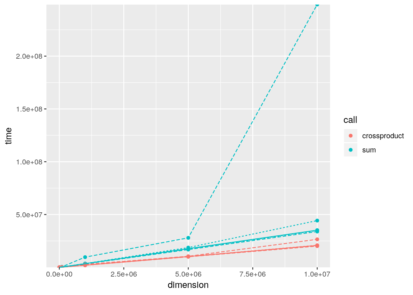
crossprod()to compute a weighted sum? How much faster is it than the naivesum(x * w)?A: We can just give the vectors to
crossprod()which converts them to row- and column-vectors and then multiplies these. The result is the dot product which is also a weighted sum.a <- rnorm(10) b <- rnorm(10) sum(a * b) - crossprod(a, b)[1] #> [1] 0A benchmark of both alternatives for different vector lengths indicates, that the
crossprod()variant is about 2.5 times faster thansum():dimensions <- c(1e1, 1e2, 1e3, 1e4, 1e5, 1e6, 0.5e7, 1e7) xvector <- lapply(dimensions, rnorm) weights <- lapply(dimensions, rnorm) bench_sum <- Map(function(x, y) fivenum(microbenchmark::microbenchmark(sum(x * y))$time), xvector, weights) bench_sum <- data.frame(time = unlist(bench_sum), call = "sum", stringsAsFactors = FALSE) bench_cp <- Map(function(x, y) fivenum(microbenchmark::microbenchmark(crossprod(x, y)[1])$time), xvector, weights) bench_cp <- data.frame(time = unlist(bench_cp), call = "crossproduct", stringsAsFactors = FALSE) df <- rbind(bench_sum, bench_cp) df$dimension <- rep(dimensions, each = 5) df$aggr <- rep(c("min", "lq", "median", "uq", "max"), times = length(dimensions)) df$aggr_size <- rep(c(1, 2, 3, 2, 1), times = length(dimensions)) df$group <- paste(as.character(df$call), as.character(df$aggr), sep = " ") library(ggplot2) ggplot(df, aes(x = dimension, y = time, colour = call, group = group)) + geom_point() + geom_line(aes(linetype = factor(aggr_size, levels = c("3", "2", "1"))), show.legend = FALSE) + scale_y_continuous(expand = c(0, 0))