13 Performance
13.1 Microbenchmarking
Q: Instead of using
microbenchmark(), you could use the built-in functionsystem.time(). Butsystem.time()is much less precise, so you’ll need to repeat each operation many times with a loop, and then divide to find the average time of each operation, as in the code below.n <- 1:1e6 system.time(for (i in n) sqrt(x)) / length(n) system.time(for (i in n) x ^ 0.5) / length(n)How do the estimates from
system.time()compare to those frommicrobenchmark()? Why are they different?Q: Here are two other ways to compute the square root of a vector. Which do you think will be fastest? Which will be slowest? Use microbenchmarking to test your answers.
x ^ (1 / 2) exp(log(x) / 2)A: The second one looks more complex, but you never know…unless you test it.
x <- runif(100) microbenchmark::microbenchmark( sqrt(x), x ^ 0.5, x ^ (1 / 2), exp(log(x) / 2) ) #> Unit: nanoseconds #> expr min lq mean median uq max neval #> sqrt(x) 312 420.0 490.59 462.0 512.0 2433 100 #> x^0.5 5605 5712.0 6096.36 5749.5 5828.5 22607 100 #> x^(1/2) 5731 5866.0 5981.55 5910.0 5985.5 8459 100 #> exp(log(x)/2) 3231 3373.5 3721.69 3447.5 3538.5 24151 100Q: Use microbenchmarking to rank the basic arithmetic operators (
+,-,*,/, and^) in terms of their speed. Visualise the results. Compare the speed of arithmetic on integers vs. doubles.A: Since I am on a Windows system, where these short execution times are hard to measure, I just ran the following code on a linux and paste the results here:
mb_integer <- microbenchmark::microbenchmark(
  1L + 1L, 1L - 1L, 1L * 1L, 1L / 1L, 1L ^ 1L,
  times = 1000000,
  control = list(order = "random",
                 warmup = 20000))

mb_double <- microbenchmark::microbenchmark(
  1 + 1, 1 - 1, 1 * 1, 1 / 1, 1 ^ 1,
  times = 1000000,
  control = list(order = "random",
                 warmup = 20000))

mb_integer
# and got the following output:
# Unit: nanoseconds
#     expr min lq      mean median uq     max neval
#  1L + 1L  50 66  96.45262     69 73 7006051 1e+06
#  1L - 1L  52 69  88.76438     71 76  587594 1e+06
#  1L * 1L  51 68  88.51854     70 75  582521 1e+06
#    1L/1L  50 65  94.40669     68 74 7241972 1e+06
#    1L^1L  67 77 102.96209     84 92  574519 1e+06

mb_double
# Unit: nanoseconds
#   expr min lq      mean median  uq      max neval
#  1 + 1  48 66  92.44331     69  75  7217242 1e+06
#  1 - 1  50 66  88.13654     68  77   625462 1e+06
#  1 * 1  48 66 135.88379     70  77 42974915 1e+06
#    1/1  48 65  87.11615     69  77   659032 1e+06
#    1^1  79 92 127.07686    103 135   641524 1e+06
To visualise and compare the results, we make some short spaghetties:
mb_median <- data.frame(operator = c("+", "-", "*", "/", "^"),
                        int = c(69, 71, 70, 68, 84),  # same as mb_integer$median
                        dbl = c(69, 68, 70, 69, 103), # same as mb_double$median
                        stringsAsFactors = FALSE)

mb_median <- tidyr::gather(mb_median, type, time, int, dbl)
mb_median <- dplyr::mutate(mb_median, type = factor(type, levels = c("int", "dbl")))

library(ggplot2)
ggplot(mb_median, aes(x = type, y = time, group = operator, color = operator)) +
  geom_point(show.legend = FALSE) +
  geom_line(show.legend = FALSE, size = 1.5) +
  geom_label(aes(label = operator), show.legend = FALSE) +
  theme_minimal() +
  ylab("time in nanoseconds") +
  theme(axis.title.x = element_blank(),
        axis.title.y = element_text(size = 14),
        axis.text.x = element_text(size = 14),
        axis.text.y = element_text(size = 10)) +
  scale_y_continuous(breaks = seq(0, max(mb_median$time), 10))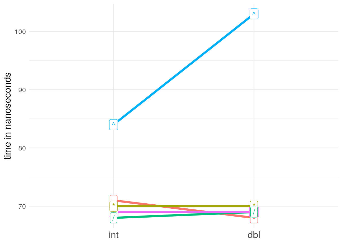
Q: You can change the units in which the microbenchmark results are expressed with the
unitparameter. Useunit = "eps"to show the number of evaluations needed to take 1 second. Repeat the benchmarks above with the eps unit. How does this change your intuition for performance?
13.2 Language performance
Q:
scan()has the most arguments (21) of any base function. About how much time does it take to make 21 promises each time scan is called? Given a simple input (e.g.,scan(text = "1 2 3", quiet = T)) what proportion of the total run time is due to creating those promises?A: According to the textbook every extra argument slows the function down by approximately 20 nanoseconds, which I can’t reproduce on my system:
f5 <- function(a = 1, b = 2, c = 4, d = 4, e = 5) NULL
f6 <- function(a = 1, b = 2, c = 4, d = 4, e = 5, f = 6) NULL
f7 <- function(a = 1, b = 2, c = 4, d = 4, e = 5, f = 6, g = 7) NULL
f8 <- function(a = 1, b = 2, c = 4, d = 4, e = 5, f = 6, g = 7, h = 8) NULL
microbenchmark::microbenchmark(f5(), f6(), f7(), f8(), times = 10000)
#> Unit: nanoseconds
#>  expr min  lq     mean median  uq    max neval
#>  f5() 245 262 455.8903    266 276 661138 10000
#>  f6() 260 280 463.3393    285 297 436882 10000
#>  f7() 277 294 509.2614    302 318 431637 10000
#>  f8() 296 317 555.9769    326 350 444821 10000
However, for now we just assume that 20 nanoseconds are correct and in kind of doubt, we recommend to benchmark this value individually. With this assumption we calculate
21 * 20 = 420nanoseconds of extra time for each call ofscan().For a percentage, we first benchmark a simple call of
scan():(mb_prom <- microbenchmark::microbenchmark( scan(text = "1 2 3", quiet = T), times = 100000, unit = "ns", control = list(warmup = 1000) )) #> Unit: nanoseconds #> expr min lq mean median uq #> scan(text = "1 2 3", quiet = T) 31353 34643 39536.45 35855 37466 #> max neval #> 14499077 1e+05 mb_prom_median <- summary(mb_prom)$medianThis lets us calculate, that ~1.17% of the median run time are caused by the extra arguments.
Q: Read “Evaluating the Design of the R Language”. What other aspects of the R-language slow it down? Construct microbenchmarks to illustrate.
Q: How does the performance of S3 method dispatch change with the length of the class vector? How does performance of S4 method dispatch change with number of superclasses? How about RC?
Q: What is the cost of multiple inheritance and multiple dispatch on S4 method dispatch?
Q: Why is the cost of name lookup less for functions in the base package?
13.3 Implementations performance
Q: The performance characteristics of
squish_ife(),squish_p(), andsquish_in_place()vary considerably with the size ofx. Explore the differences. Which sizes lead to the biggest and smallest differences?Q: Compare the performance costs of extracting an element from a list, a column from a matrix, and a column from a data frame. Do the same for rows.